Working with unstructured meshes in xESMF

xESMF can now build regridders from UGRID-style unstructured mesh inputs using mesh_in=True. This makes it possible to regrid face-centered data from an unstructured source mesh to a structured output grid. For real-world unstructured mesh files, we recommend using UXarray to read the mesh and normalize its topology metadata into a consistent UGRID-style representation before passing it to xESMF. UXarray is used in this notebook only as a convenient way to load public example meshes; xESMF itself consumes xarray datasets with mesh coordinates and connectivity.

Currently supported:

Face-centered source data on mesh faces.
Mesh-to-structured-grid regridding.
Spherical longitude/latitude mesh coordinates.
Cartesian xyz mesh coordinates.
bilinear, patch, nearest_s2d, and nearest_d2s methods.
UGRID-style _FillValue and start_index metadata on face-node connectivity.

Not yet supported:

Node-centered source data.
Edge-centered source data.
Mixed node/face coordinate geometry modes.
Conservative mesh regridding methods.
Mesh output grids.

[1]:

import numpy as np
import xarray as xr
import uxarray as ux
import xesmf as xe
import matplotlib.pyplot as plt

Download example mesh files

This notebook uses small public example files from the UXarray repository. The helper below downloads each file once and reuses it from a local cache on subsequent runs, so the example data do not need to be stored in the xESMF repository.

If you prefer, you can also download these files manually from the UXarray repository and pass the local file paths directly to ux.open_dataset.

[2]:

from pathlib import Path
from urllib.request import urlretrieve

CACHE_DIR = Path.home() / ".cache" / "xesmf-uxarray"
CACHE_DIR.mkdir(parents=True, exist_ok=True)


def fetch_uxarray_example(filename, base_url):
    """Download a UXarray example file once and reuse it from a local cache."""
    local_path = CACHE_DIR / filename
    if not local_path.exists():
        url = f"{base_url.rstrip('/')}/{filename}"
        print(f"Downloading {url}")
        urlretrieve(url, local_path)
    return local_path

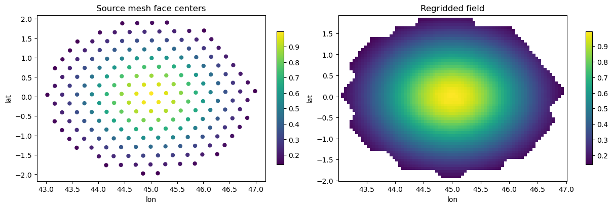
Regridding a small MPAS example mesh

We start with a small subset of a 30 km MPAS atmosphere mesh from the UXarray example data repository. The example consists of a separate grid file and data file. UXarray reads the MPAS files and exposes the mesh in a normalized form with face centers, node coordinates, and face-node connectivity.

The data file contains face-centered example fields, including gaussian and inverse_gaussian, which makes it a compact test case for regridding from an unstructured mesh to a structured latitude-longitude grid.

[3]:

base_url = "https://raw.githubusercontent.com/UXARRAY/uxarray/main/test/meshfiles/mpas/dyamond-30km"

grid_path = fetch_uxarray_example("gradient_grid_subset.nc", base_url)
data_path = fetch_uxarray_example("gradient_data_subset.nc", base_url)

uxds = ux.open_dataset(grid_path, data_path)
uxds.data_vars

[3]:

Data variables:
    face_lat          (n_face) float32 780B ...
    face_lon          (n_face) float32 780B ...
    gaussian          (n_face) float32 780B ...
    inverse_gaussian  (n_face) float32 780B ...

Next, we define a simple structured latitude-longitude target grid covering the same longitude and latitude range as the source mesh. This will be the grid that the unstructured face-centered data are regridded onto.

[4]:

lon = np.linspace(
    float(uxds.uxgrid.face_lon.values.min()),
    float(uxds.uxgrid.face_lon.values.max()),
    80,
)
lat = np.linspace(
    float(uxds.uxgrid.face_lat.values.min()),
    float(uxds.uxgrid.face_lat.values.max()),
    60,
)

dst = xr.Dataset(
    coords={
        "lon": ("lon", lon),
        "lat": ("lat", lat),
    }
)
dst

[4]:

<xarray.Dataset> Size: 1kB
Dimensions:  (lon: 80, lat: 60)
Coordinates:
  * lon      (lon) float64 640B 43.03 43.08 43.13 43.18 ... 46.88 46.93 46.98
  * lat      (lat) float64 480B -1.98 -1.914 -1.848 -1.783 ... 1.772 1.838 1.903
Data variables:
    *empty*

[5]:

regridder = xe.Regridder(
    uxds,
    dst,
    "bilinear",
    mesh_in=True,
    unmapped_to_nan=True,
)
out = regridder(uxds["gaussian"])

[6]:

fig, axes = plt.subplots(1, 2, figsize=(12, 4), constrained_layout=True)

sc = axes[0].scatter(
    uxds.uxgrid.face_lon.values,
    uxds.uxgrid.face_lat.values,
    c=uxds["gaussian"].values,
    s=25,
    cmap="viridis",
)
axes[0].set_title("Source mesh face centers")
axes[0].set_xlabel("lon")
axes[0].set_ylabel("lat")
plt.colorbar(sc, ax=axes[0], shrink=0.8)

pcm = axes[1].pcolormesh(
    dst["lon"].values,
    dst["lat"].values,
    out.values,
    shading="auto",
    cmap="viridis",
)
axes[1].set_title("Regridded field")
axes[1].set_xlabel("lon")
axes[1].set_ylabel("lat")
plt.colorbar(pcm, ax=axes[1], shrink=0.8)

[6]:

<matplotlib.colorbar.Colorbar at 0x1770afcb0>

../_images/notebooks_Unstructured_grid_9_1.png

Working with unstructured meshes in xESMF

Download example mesh files

Regridding a small MPAS example mesh

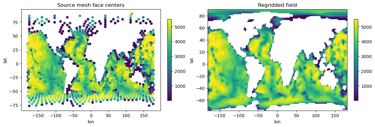
Regridding a larger MPAS-Ocean mesh

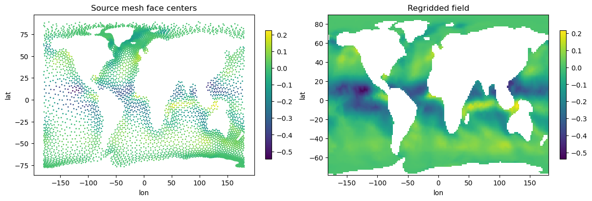
Regridding a FESOM field

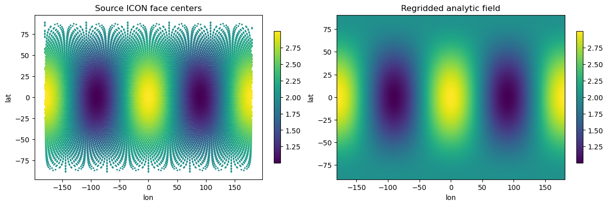
Regridding an ICON mesh