Regrid between rectilinear grids
[1]:
%matplotlib inline
import matplotlib.pyplot as plt
import cartopy.crs as ccrs
import numpy as np
import xarray as xr
import xesmf as xe
Prepare data
Input data
We regrid xarray’s built-in demo data. This data is also used by xarray plotting tutorial.
[2]:
ds = xr.tutorial.open_dataset(
    "air_temperature"
)  # use xr.tutorial.load_dataset() for xarray<v0.11.0
ds
[2]:
<xarray.Dataset>
Dimensions:  (lat: 25, time: 2920, lon: 53)
Coordinates:
  * lat      (lat) float32 75.0 72.5 70.0 67.5 65.0 ... 25.0 22.5 20.0 17.5 15.0
  * lon      (lon) float32 200.0 202.5 205.0 207.5 ... 322.5 325.0 327.5 330.0
  * time     (time) datetime64[ns] 2013-01-01 ... 2014-12-31T18:00:00
Data variables:
    air      (time, lat, lon) float32 ...
Attributes:
    Conventions:  COARDS
    title:        4x daily NMC reanalysis (1948)
    description:  Data is from NMC initialized reanalysis\n(4x/day).  These a...
    platform:     Model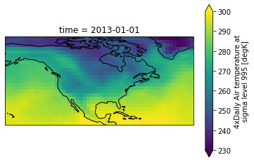
references: http://www.esrl.noaa.gov/psd/data/gridded/data.ncep.reanaly...It is the air temperature data over US with 2920 time frames. Let’s plot the first frame:
[3]:
dr = ds["air"] # get a DataArray
[4]:
ax = plt.axes(projection=ccrs.PlateCarree())
dr.isel(time=0).plot.pcolormesh(ax=ax, vmin=230, vmax=300)
ax.coastlines()
[4]:
<cartopy.mpl.feature_artist.FeatureArtist at 0x7f3923d7f400>
Input grid
Its grid resolution is \(2.5^\circ \times 2.5^\circ\):
[5]:
ds["lat"].values, ds["lon"].values
[5]:
(array([75. , 72.5, 70. , 67.5, 65. , 62.5, 60. , 57.5, 55. , 52.5, 50. ,
47.5, 45. , 42.5, 40. , 37.5, 35. , 32.5, 30. , 27.5, 25. , 22.5,
20. , 17.5, 15. ], dtype=float32),
array([200. , 202.5, 205. , 207.5, 210. , 212.5, 215. , 217.5, 220. ,
222.5, 225. , 227.5, 230. , 232.5, 235. , 237.5, 240. , 242.5,
245. , 247.5, 250. , 252.5, 255. , 257.5, 260. , 262.5, 265. ,
267.5, 270. , 272.5, 275. , 277.5, 280. , 282.5, 285. , 287.5,
290. , 292.5, 295. , 297.5, 300. , 302.5, 305. , 307.5, 310. ,
312.5, 315. , 317.5, 320. , 322.5, 325. , 327.5, 330. ],
dtype=float32))
Output grid
Say we want to downsample it to \(1.0^\circ \times 1.5^\circ\). Just define the output grid as an xarray Dataset. Notice here that we take care of passing some attributes to the coordinate variables. This ensures xESMF and it’s underlying helper, cf-xarray, understand which is which.
[6]:
ds_out = xr.Dataset(
{
"lat": (["lat"], np.arange(16, 75, 1.0), {"units": "degrees_north"}),
"lon": (["lon"], np.arange(200, 330, 1.5), {"units": "degrees_east"}),
}
)
ds_out
[6]:
<xarray.Dataset>
Dimensions: (lat: 59, lon: 87)
Coordinates:
* lat (lat) float64 16.0 17.0 18.0 19.0 20.0 ... 70.0 71.0 72.0 73.0 74.0
* lon (lon) float64 200.0 201.5 203.0 204.5 ... 324.5 326.0 327.5 329.0
Data variables:
*empty*Perform regridding
Make a regridder by xe.Regridder(grid_in, grid_out, method). grid is just an xarray Dataset containing lat and lon values. In most cases, 'bilinear' should be good enough. For other methods see Comparison of 5 regridding algorithms.
[7]:
regridder = xe.Regridder(ds, ds_out, "conservative")
regridder # print basic regridder information.
[7]:
xESMF Regridder
Regridding algorithm: conservative
Weight filename: conservative_25x53_59x87.nc
Reuse pre-computed weights? False
Input grid shape: (25, 53)
Output grid shape: (59, 87)
Periodic in longitude? False
The regridder says it can transform data from shape (25, 53) to shape (59, 87).
Regrid the DataArray is straightforward:
[8]:
dr_out = regridder(dr, keep_attrs=True)
dr_out
[8]:
<xarray.DataArray 'air' (time: 2920, lat: 59, lon: 87)>
array([[[296.1936 , 296.4933 , 296.64383, ..., 296.6239 , 296.57 ,
296.35767],
[295.9 , 296.09998, 296.19998, ..., 295.9 , 295.9 ,
295.43332],
[295.9 , 296.09998, 296.19998, ..., 295.9 , 295.9 ,
295.43332],
...,
[243.79999, 244.26666, 244.5 , ..., 233.63335, 235.29999,
237.96663],
[243.79999, 244.26666, 244.5 , ..., 233.63335, 235.29999,
237.96663],
[241.87102, 242.6313 , 243.01498, ..., 233.68292, 235.44838,
237.66943]],
[[296.26776, 296.8064 , 297.0761 , ..., 296.19287, 296.17752,
296.2103 ],
[296.19998, 296.53333, 296.69998, ..., 295.56668, 295.5 ,
295.23334],
[296.19998, 296.53333, 296.69998, ..., 295.56668, 295.5 ,
295.23334],
...
[249.89 , 249.49 , 249.29 , ..., 241.69 , 242.48999,
243.68997],
[249.89 , 249.49 , 249.29 , ..., 241.69 , 242.48999,
243.68997],
[246.84814, 246.2443 , 245.9487 , ..., 243.05266, 243.60286,
244.30954]],
[[297.2945 , 297.6252 , 297.79266, ..., 296.21606, 296.0664 ,
295.7324 ],
[296.09 , 296.62332, 296.88998, ..., 295.69 , 295.69 ,
295.35666],
[296.09 , 296.62332, 296.88998, ..., 295.69 , 295.69 ,
295.35666],
...,
[249.89 , 249.49 , 249.29 , ..., 239.82333, 240.29 ,
241.22331],
[249.89 , 249.49 , 249.29 , ..., 239.82333, 240.29 ,
241.22331],
[246.3288 , 245.82306, 245.57744, ..., 241.16115, 241.18028,
241.57034]]], dtype=float32)
Coordinates:
* time (time) datetime64[ns] 2013-01-01 ... 2014-12-31T18:00:00
* lon (lon) float64 200.0 201.5 203.0 204.5 ... 324.5 326.0 327.5 329.0
* lat (lat) float64 16.0 17.0 18.0 19.0 20.0 ... 70.0 71.0 72.0 73.0 74.0
Attributes:
long_name: 4xDaily Air temperature at sigma level 995
units: degK
precision: 2
GRIB_id: 11
GRIB_name: TMP
var_desc: Air temperature
dataset: NMC Reanalysis
level_desc: Surface
statistic: Individual Obs
parent_stat: Other
actual_range: [185.16 322.1 ]
regrid_method: conservativeThe horizontal shape is now (59, 87), as expected. The regridding operation broadcasts over extra dimensions (time here), so there are still 2920 time frames. lon and lat coordinate values are updated accordingly, and the value of the extra dimension time is kept the same as input.
Important note: Extra dimensions must be on the left, i.e. (time, lev, lat, lon) is correct but (lat, lon, time, lev) would not work. Most data sets should have (lat, lon) on the right (being the fastest changing dimension in the memory). If not, use DataArray.transpose or numpy.transpose to preprocess the data.
Check results on 2D map
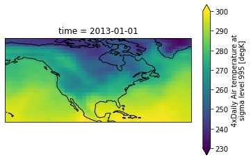
The regridding result is consistent with the original data, with a much finer resolution:
[9]:
ax = plt.axes(projection=ccrs.PlateCarree())
dr_out.isel(time=0).plot.pcolormesh(ax=ax, vmin=230, vmax=300)
ax.coastlines()
[9]:
<cartopy.mpl.feature_artist.FeatureArtist at 0x7f391ace9eb0>
Check broadcasting over extra dimensions
xESMF tracks coordinate values over extra dimensions, since horizontal regridding should not affect them.
[10]:
dr_out["time"]
[10]:
<xarray.DataArray 'time' (time: 2920)>
array(['2013-01-01T00:00:00.000000000', '2013-01-01T06:00:00.000000000',
       '2013-01-01T12:00:00.000000000', ..., '2014-12-31T06:00:00.000000000',
       '2014-12-31T12:00:00.000000000', '2014-12-31T18:00:00.000000000'],
      dtype='datetime64[ns]')
Coordinates:
* time (time) datetime64[ns] 2013-01-01 ... 2014-12-31T18:00:00
Attributes:
standard_name: time
long_name: Time[11]:
# exactly the same as input
xr.testing.assert_identical(dr_out["time"], ds["time"])
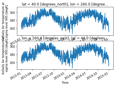
We can plot the time series at a specific location, to make sure the broadcasting is correct:
[12]:
plt.subplot(2, 1, 1)
dr.sel(lon=260, lat=40).plot()  # input data
plt.subplot(2, 1, 2)
dr_out.sel(lon=260, lat=40).plot()  # output data
[12]:
[<matplotlib.lines.Line2D at 0x7f391ac417c0>]